FPGA图像处理中常用的图像缩放算法,包括最近邻插值算法、双线性邻插值算法、双三次邻插值算法,以及双线性的MATLAB与FPGA实现。
双线性邻域插值算法
基础理论
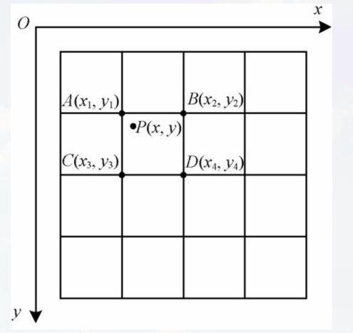
核心思想: 标准的线性插值是在一维直线上,根据已知两点的坐标和值,来计算中间某个未知点的值。而双线性插值指的是做了两次线性插值,是在一个二维平面上的。而 双线性插值 (Bilinear Interpolation),顾名思义,就是做了两次线性插值,但它是在一个二维平面上。当我们要计算目标图像中某个点 (x, y) 的像素值时,我们先找到它对应在源图像中的位置 (src_x, src_y)。这个位置通常是浮点数,落在四个真实像素点之间。
算法步骤:
- 坐标映射:将目标图像的坐标
(dst_x, dst_y) 映射回源图像的坐标 (src_x, src_y)。
- 找到四个邻近点:根据
(src_x, src_y) 找到它周围的四个像素点,即上图的 Q11, Q12, Q21, Q22。(如上图)
- 第一次线性插值:在 x 方向上,分别对上下两行进行线性插值,计算出两个临时点
R1 和 R2 的值。
- 第二次线性插值:在 y 方向上,对
R1 和 R2 进行线性插值,最终得到 P 点的像素值。
公式:
f(P) = (1 - d_x)(1 - d_y) f(Q_{11}) + d_x(1 - d_y) f(Q_{21}) + (1 - d_x)d_y f(Q_{12}) + d_x d_y f(Q_{22})
原理实例化:
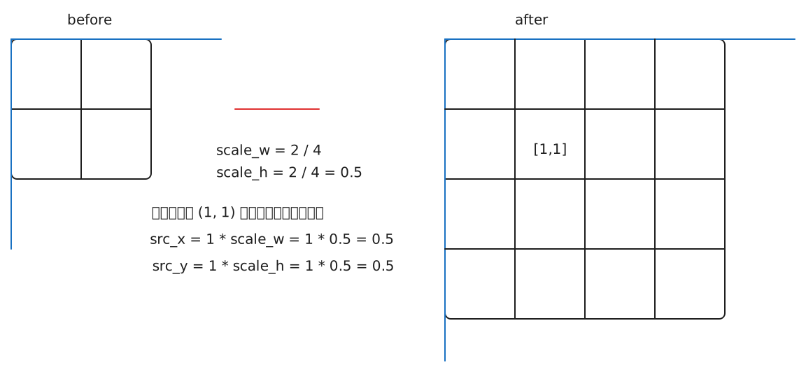
笔者理论改进
笔者最终目标是实现再FPGA可以高效运行的双线性插值,为此需要在一开始从算法层面去改进。出于习惯,个人觉得以下公式更清晰:
I(i, j) = [1 - y(i)] \times \left\{ [(1 - x(j)) \times T_A(r) + x(j) \times T_B(r)] \right\} + y(i) \times \left\{ [(1 - x(j)) \times T_C(r) + x(j) \times T_D(r)] \right\}
为了清晰地表达,约定以下符号:
- **Ws,Hs**:源图像的宽度和高度。
- **Wd,Hd**:目标图像的宽度和高度。
- **(dstx,dsty)**:目标图像中的像素坐标。
- **(srcx,srcy)**:通过映射在源图像中得到的浮点坐标。
- **(x1,y1)**:包围 (srcx,srcy) 的四点矩阵的左上角整数坐标,即 x1=⌊srcx⌋,y1=⌊srcy⌋。
- **dx,dy**:浮点坐标的小数部分,即 dx=srcx−x1,dy=srcy−y1。
- **N**:定点运算的小数位数,这里 N=10。
- **S**:缩放因子 (Scale),S=2N=1024。
- **Xfixed**:表示变量 X 的定点整数形式。
- **TA,TB,TC,TD**:分别代表源图像中四个邻近像素 f(x1,y1), f(x1+1,y1), f(x1,y1+1), f(x1+1,y1+1) 的值。
- **≪N**:代表逻辑左移N位(乘以 S=2N)。
- **≫N**:代表算术右移N位(除以 S=2N 并向下取整)。
改进1:
小数在FPGA中是难以接受的,所以将1扩大1024倍,为此得到
I(i, j) = [1024 - y(i)] \times \left\{ [(1024 - x(j)) \times T_A(r) + x(j) \times T_B(r)] \right\} + y(i) \times \left\{ [(1024 - x(j)) \times T_C(r) + x(j) \times T_D(r)] \right\}
改进2:
上述公式存在6次乘法,而且在实际中位宽较大,比较消耗资源,为此采取差分方式来代替上述表达式,差分情况下只需要做三次乘法,对于1024的除法采用移位即可。
I(i,j)\;=\;
\bigl(1024-y(i)\bigr)\Bigl[T_A(r)+\bigl(T_B(r)-T_A(r)\bigr)\tfrac{x(j)}{1024}\Bigr]
\;+\;
y(i)\Bigl[T_C(r)+\bigl(T_D(r)-T_C(r)\bigr)\tfrac{x(j)}{1024}\Bigr]
## 分步数学推导
### 前处理 / 地址生成单元
这部分的目标是根据目标像素坐标 `(dst_x, dst_y)`,计算出插值所需的四个源像素位置和两个权重。
**1. 坐标映射:**
将目标坐标范围 `[0, Wd-1]` 映射到源坐标范围 `[0, Ws-1]`。
标准浮点公式:
\begin{align*}
src_x &= dst_x \cdot \frac{W_s - 1}{W_d - 1} \\
src_y &= dst_y \cdot \frac{H_s - 1}{H_d - 1}
\end{align*}
定点实现公式:
\begin{align*}
src\_x_{fixed} &= \left\lfloor \frac{dst_x \cdot (W_s - 1) \cdot S}{W_d - 1} \right\rfloor \\
src\_y_{fixed} &= \left\lfloor \frac{dst_y \cdot (H_s - 1) \cdot S}{H_d - 1} \right\rfloor
\end{align*}
**2. 分解整数坐标与小数权重**
从定点坐标 `src_x_fixed` 中分离出整数部分 `x1` 和归一化的小数权重 `x_norm`。
整数坐标 `x1,y1` 公式:
\begin{align*}
x_1 &= \left\lfloor \frac{src\_x_{fixed}}{S} \right\rfloor \quad \Leftrightarrow \quad x_1 = src\_x_{fixed} \gg N \\
y_1 &= \left\lfloor \frac{src\_y_{fixed}}{S} \right\rfloor \quad \Leftrightarrow \quad y_1 = src\_y_{fixed} \gg N
\end{align*}
小数坐标`x_norm` ,`y_norm`公式:
\begin{align*}
dx &= src_x - x_1 \implies dx_{fixed} = (src_x - x_1) \cdot S = src\_x_{fixed} - x_1 \cdot S \\
x_{norm} &= src\_x_{fixed} \pmod{S} \quad \Leftrightarrow \quad x_{norm} = src\_x_{fixed} \,\&\, (S - 1)
\end{align*}
y_norm 同理
插值计算核心
省流:为什么这么做?因为这个版本逻辑对于fpga来说既能保持精度(与浮点存在±1误差),又符合计算逻辑
1
2
3
| // R1 = TA << 10 + x * (TB - TA)
// R2 = TC << 10 + x * (TD - TC)
// I = R1 >> 10 + [y * (R2 - R1)] >> 20
|
1. X方向的线性插值
计算中间点 R1 (在 y1 行) 和 R2 (在 y1+1 行) 的值。
标准浮点公式:
\begin{align*}
R_1 &= (1 - dx) \cdot TA + dx \cdot TB \\
R_2 &= (1 - dx) \cdot TC + dx \cdot TD
\end{align*}
定点公式:
R_{1_{fixed}} = (S - x_{norm}) \cdot TA + x_{norm} \cdot TB
展开
R\_1_{fixed} = S \cdot TA - x_{norm} \cdot TA + x_{norm} \cdot TB = (TA \ll N) + x_{norm} \cdot (TB - TA)
R_2fix同理
**2. Y方向的线性插值**
利用 R1 和 R2 计算最终像素值 I。
标准浮点公式:
I = (1 - dy) \cdot R_1 + dy \cdot R_2
定点实现公式:
I_{final} = \left\lfloor \frac{(S - y_{norm}) \cdot R_{1_{fixed}} + y_{norm} \cdot R_{2_{fixed}}}{S^2} \right\rfloor
拆分展开:
\begin{align*}
I_{final} &= \left\lfloor \frac{S \cdot R_{1_{fixed}} + y_{norm} \cdot (R_{2_{fixed}} - R_{1_{fixed}})}{S^2} \right\rfloor \\
I_{final} &= \left\lfloor \frac{R_{1_{fixed}}}{S} + \frac{y_{norm} \cdot (R_{2_{fixed}} - R_{1_{fixed}})}{S^2} \right\rfloor
\end{align*}
**3. 最终步骤**
I_{final} = (R_{1_{fixed}} \gg N) + \left( (y_{norm} \cdot (R_{2_{fixed}} - R_{1_{fixed}})) \gg 2N \right)
## python定点实现
### code
1
2
3
4
5
6
7
8
9
10
11
12
13
14
15
16
17
18
19
20
21
22
23
24
25
26
27
28
29
30
31
32
33
34
35
36
37
38
39
40
41
42
43
44
45
46
47
48
49
50
51
52
53
54
55
56
57
58
59
60
61
62
63
64
65
66
67
68
69
70
71
72
73
74
75
76
77
78
79
80
81
82
83
84
85
86
87
88
89
90
91
92
93
94
95
96
97
98
99
100
101
102
103
104
105
106
107
108
| import cv2
import numpy as np
import numpy as ny
import matplotlib.pyplot as plt
from scipy.stats import yeojohnson_normmax
matplotlib.rcParams['font.sans-serif'] = ['SimHei']
matplotlib.rcParams['axes.unicode_minus'] = False
def bilinear_verilog(src_img,dst_shape):
FRAC_BITS = 10
SCALE = 1 << FRAC_BITS
src_h,src_w = src_img.shape[:2]
dst_h,dst_w = dst_shape
if len(src_img.shape) == 3:
channels = src_img.shape[2]
else:
channels =1
dst_img = np.zeros((dst_h,dst_w,channels),np.uint8)
for dst_y in range(dst_h):
for dst_x in range(dst_w):
src_x_fixed = (dst_x * (src_w-1) * SCALE)//(dst_w-1)
src_h_fixed = (dst_y * (src_h-1) * SCALE)//(dst_h-1)
x1 = src_x_fixed >> FRAC_BITS
y1 = src_h_fixed >> FRAC_BITS
x_norm = src_x_fixed & (SCALE-1)
y_norm = src_h_fixed & (SCALE-1)
x2 = x1 + 1
y2 = y1 + 1
x1 = max(0, x1);x2 = min(src_w - 1, x2)
y1 = max(0, y1);y2 = min(src_h - 1, y2)
for c in range(channels):
TA = int(src_img[y1,x1,c])
TB = int(src_img[y1,x2,c])
TC = int(src_img[y2, x1, c])
TD = int(src_img[y2, x2, c])
diff1 = TB - TA
diff2 = TD - TC
R1 = (TA << FRAC_BITS) + x_norm * diff1
R2 = (TB << FRAC_BITS) + x_norm * diff2
term1 = R1 >> FRAC_BITS
diff_R = R2 - R1
mult_v = y_norm * diff_R
rounding_offset = 1 << (2 * FRAC_BITS - 1)
term2 = (mult_v + rounding_offset) >> (2 * FRAC_BITS)
final_pixel_val = term1 + term2
dst_img[dst_y, dst_x, c] = np.clip(final_pixel_val,0,255)
if channels == 1:
dst_img = np.squeeze(dst_img, axis=2)
return dst_img
if __name__=='__main__':
img = cv2.imread('tenshu.jpg')
img = cv2.cvtColor(img,cv2.COLOR_BGR2RGB)
target_shape = (480,640)
zoomed_verilog = bilinear_verilog(img,target_shape)
target_size_cv2 = (target_shape[1], target_shape[0])
zoomed_cv2 = cv2.resize(img,target_size_cv2,interpolation=cv2.INTER_LINEAR)
plt.figure(figsize=(15, 7))
plt.suptitle("Verilog风格定点实现 vs OpenCV实现", fontsize=16)
plt.subplot(1, 3, 1)
plt.imshow(img)
plt.title(f"原始图像 ({img.shape[1]}x{img.shape[0]})")
plt.subplot(1, 3, 2)
plt.imshow(zoomed_verilog)
plt.title(f"Verilog风格定点实现 ({target_shape[1]}x{target_shape[0]})")
plt.subplot(1, 3, 3)
plt.imshow(zoomed_cv2)
plt.title(f"OpenCV cv2.resize")
plt.tight_layout(rect=[0, 0.03, 1, 0.95])
plt.show()
|
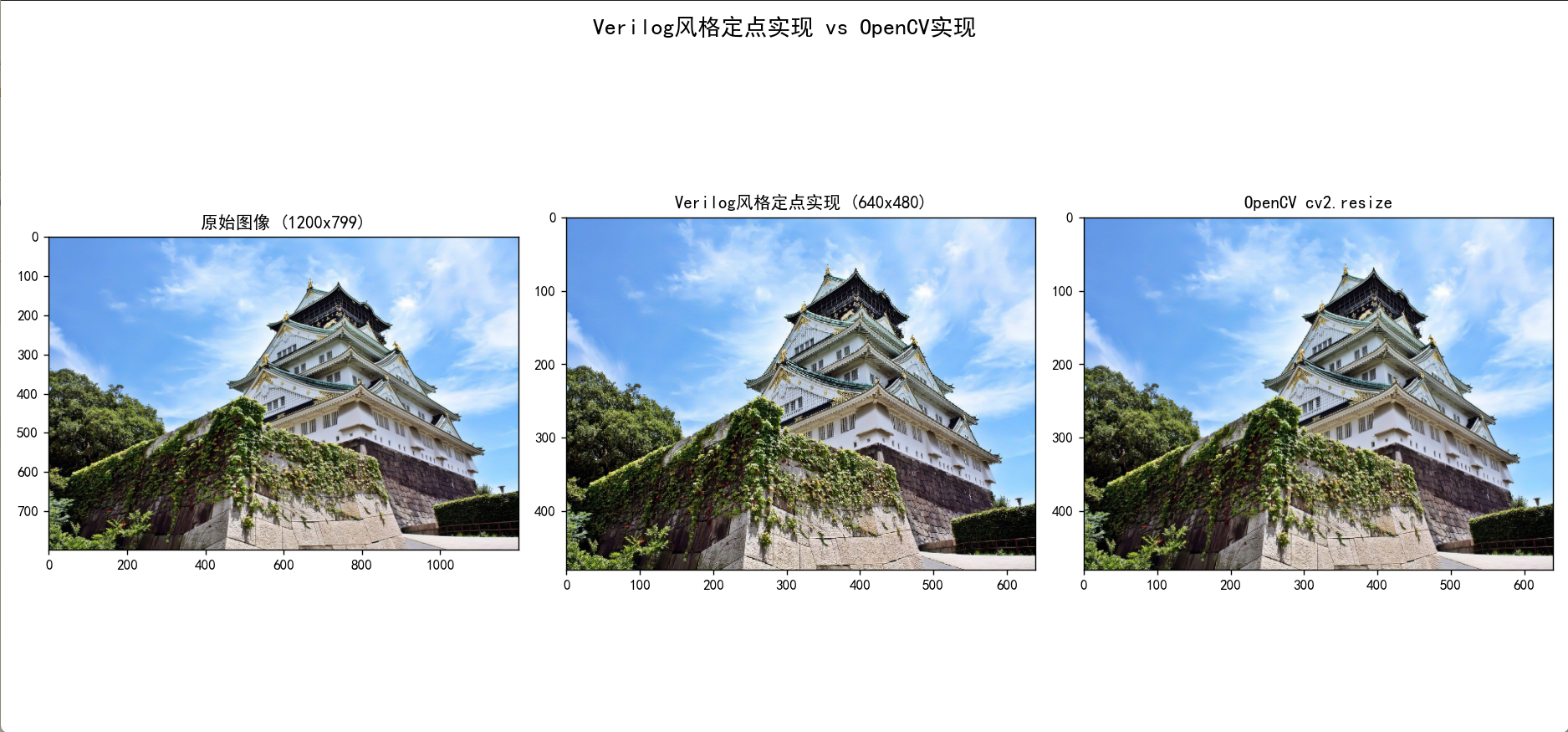
result
优化
除法计算过于多,每个像素都进行一次除法,这是极其反优化的。为此优化只做一次,预先计算一个高精度的“组合缩放因子”,这个因子包含了原始的缩放比例和用于最终结果的SCALE。
1
2
3
4
5
6
7
8
9
10
11
12
13
14
15
16
17
18
19
20
21
22
23
24
25
26
27
28
29
30
31
32
33
34
35
36
37
38
39
40
41
42
43
44
45
46
47
48
49
50
51
52
53
54
55
56
57
58
59
60
61
62
63
64
65
66
67
68
69
70
71
72
73
74
75
76
77
78
79
80
81
82
83
84
85
86
87
88
89
90
91
92
93
94
95
96
97
98
99
100
101
102
103
104
105
106
107
108
109
110
111
112
113
114
115
116
117
118
119
120
121
122
123
124
125
126
|
import cv2
import numpy as np
import matplotlib.pyplot as plt
matplotlib.rcParams['font.sans-serif'] = ['SimHei']
matplotlib.rcParams['axes.unicode_minus'] = False
def bilinear_verilog_optimized(src_img, dst_shape):
SCALE = 1 << FRAC_BITS
dst_h, dst_w = dst_shape
if len(src_img.shape) == 3:
channels = src_img.shape[2]
else:
channels = 1
src_img = np.expand_dims(src_img, axis=-1)
dst_img = np.zeros((dst_h, dst_w, channels), np.uint8)
RATIO_PRECISION_BITS = 16
RATIO_SCALE = 1 << RATIO_PRECISION_BITS
if dst_w > 1:
combined_scale_x = ((src_w - 1) * SCALE * RATIO_SCALE) // (dst_w - 1)
else:
combined_scale_x = 0
if dst_h > 1:
combined_scale_y = ((src_h - 1) * SCALE * RATIO_SCALE) // (dst_h - 1)
else:
combined_scale_y = 0
for dst_x in range(dst_w):
src_x_fixed = (dst_x * combined_scale_x) >> RATIO_PRECISION_BITS
src_y_fixed = (dst_y * combined_scale_y) >> RATIO_PRECISION_BITS
y1 = src_y_fixed >> FRAC_BITS
x_norm = src_x_fixed & (SCALE - 1)
y_norm = src_y_fixed & (SCALE - 1)
y2 = y1 + 1
x1 = max(0, x1); x2 = min(src_w - 1, x2)
y1 = max(0, y1); y2 = min(src_h - 1, y2)
TA = int(src_img[y1, x1, c])
TB = int(src_img[y1, x2, c])
TC = int(src_img[y2, x1, c])
TD = int(src_img[y2, x2, c])
diff1 = TB - TA
diff2 = TD - TC
R1 = (TA << FRAC_BITS) + x_norm * diff1
R2 = (TC << FRAC_BITS) + x_norm * diff2
term1 = R1 >> FRAC_BITS
diff_R = R2 - R1
mult_v = y_norm * diff_R
rounding_offset = 1 << (2 * FRAC_BITS - 1)
term2 = (mult_v + rounding_offset) >> (2 * FRAC_BITS)
final_pixel_val = term1 + term2
dst_img[dst_y, dst_x, c] = np.clip(final_pixel_val, 0, 255)
if channels == 1:
dst_img = np.squeeze(dst_img, axis=-1)
return dst_img
try:
img = cv2.imread('tenshu.jpg')
img = cv2.cvtColor(img, cv2.COLOR_BGR2RGB)
except Exception as e:
print(f"无法加载图像 'tenshu.jpg',请确保文件存在。错误: {e}")
img = np.zeros((100, 100, 3), dtype=np.uint8)
img[0:50, 0:50] = [255, 0, 0]
img[50:100, 0:50] = [0, 255, 0]
img[0:50, 50:100] = [0, 0, 255]
img[50:100, 50:100] = [255, 255, 0]
target_shape = (480, 640)
zoomed_verilog = bilinear_verilog_optimized(img, target_shape)
target_size_cv2 = (target_shape[1], target_shape[0])
zoomed_cv2 = cv2.resize(img, target_size_cv2, interpolation=cv2.INTER_LINEAR)
plt.figure(figsize=(15, 7))
plt.suptitle("优化后的定点实现 vs OpenCV实现", fontsize=16)
plt.subplot(1, 3, 1)
plt.imshow(img)
plt.title(f"原始图像 ({img.shape[1]}x{img.shape[0]})")
plt.subplot(1, 3, 2)
plt.imshow(zoomed_verilog)
plt.title(f"优化后的定点实现 ({target_shape[1]}x{target_shape[0]})")
plt.subplot(1, 3, 3)
plt.imshow(zoomed_cv2)
plt.title(f"OpenCV cv2.resize")
plt.tight_layout(rect=[0, 0.03, 1, 0.95])
plt.show()
|
FPGA实现
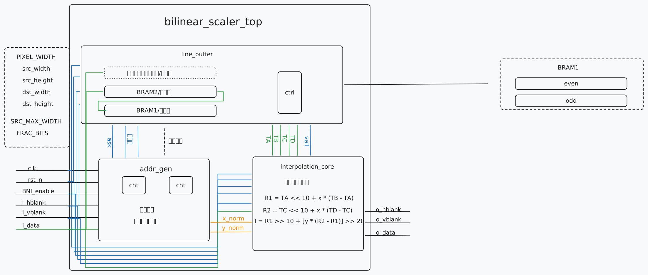
模块设计
BUG日志
“今天又在很努力的写bug了!”
在Verilog实现地址生成的过程中,难以避免对于除法精度的处理
如下公式,往往会出现小数,就算对其扩大,由于dst也是较大的数字,一旦误差被放大1000也是巨大的偏移,会越来越偏,花了大半天时间,很难在资源和效率之间平衡,每次都用除法资源量是巨大的,不可接受!!又想着去修正数值,但是这样又会写死,难以适配更多的变化。
最后,取消了-1 🤤,不可否认的是这样也存在难以适配的问题,但是这也许是当先最简单最省事最可靠的办法,对于其它分辨率变化,我认为更应该是在 localparam 部分就让他为整数。
\begin{align*}
src_x &= dst_x \cdot \frac{W_s - 1}{W_d - 1} \\
src_y &= dst_y \cdot \frac{H_s - 1}{H_d - 1}
\end{align*}